On Biological Data Generation 2/n: The Economics of Metrology

What to measure, what a measurement preserves, and what it costs to make an observation identifiable

In 1/n, I used Philip Anderson’s “More Is Different” as a starting point for thinking about the generation of biological data. Anderson accepted that higher-order systems obey the laws governing their constituent parts. His harder point was that those laws do not automatically supply the effective variables needed to describe the organized system above them. A cell obeys molecular physics, but a useful cellular description does not emerge simply by listing every molecule. As the organization changes, the observables required to explain the behavior change with it. DOI.org

Michael Bronstein and Luca Naef extend this argument in a complementary direction. Their “black-box data” framework questions whether biological measurements should continue to be designed mainly for human interpretation without aid, or if some data sources should be optimized for machine learning instead: higher throughput, less immediate interpretability, and more algorithmic processing between raw measurement and the desired outcome. Importantly, the black box refers to the inverse problem between measurement and useful output, not to any relaxation of experimental rigor. The measurement still needs to contain enough signal, metadata, calibration, and structure for that inverse problem to be solvable. Royal Society of Chemistry Publications

That brings the argument into metrology—the science of measurement and its application—and then one step further into the economics of metrology. Metrology conventionally includes calibration, reference standards, uncertainty, quality assurance, and traceability. The economic layer accounts for what a measurement resolves, what it averages, which structures survive the measurement, and how much downstream work is required before the resulting observation becomes useful. This is a useful conceptual extension without straying from the technical core of the discipline. NIST

Most assay comparisons begin with cost per sample because it is visible, procurement-friendly, and easy to place in a spreadsheet. Reagents, sample preparation, instrument time, sequencing, imaging, labor, compute, and storage can all be assigned numbers. That ledger is necessary, but incomplete. The differentiators are at a higher level of abstraction. An assay can win the spreadsheet by removing the structure that made the underlying question identifiable. Therefore the cost then reemerges downstream as extra modalities, more disturbances, more replicates, stronger modeling assumptions, or a model that fails outside the conditions in which it was trained.

Bulk sequencing is the canonical example. It was transformative because it scaled. DNA was an unusually favorable substrate: stable, linear, amplifiable [Nobel][https://www.nobelprize.org/prizes/chemistry/1993/summary/], and readable [Nobel][https://www.nobelprize.org/prizes/chemistry/1980/summary/]. But bulk measurement also averages; it collapses cell identity, spatial position, local exchange, neighborhood, topology, and time. That was very useful early on and has given us many, many advances, but we tend to forget that we’re looking at aggregate measures/statistical ensembles. It’s much less useful when the questions to be answered concern organization, communication, perturbation response, or decision-making.

The unit I want to reason about is therefore the cost per task-relevant, identifiable observation. An observation is identifiable when it preserves enough of the relevant state and context that the latent variable, transition, or mechanism can be inferred without a cascade of heroic assumptions. In current machine-learning parlance, such an observation may serve as a useful training example, but actually, we don’t want to be constrained to today’s training paradigm. Rather, we recognize and celebrate that the scientific object is broader: it may be useful to constrain a mechanistic model, a causal graph, a Bayesian inference procedure, a dynamical simulator, or a control policy. So let’s get into it!

A first-pass cost accounting might look like:

C_identifiable ≈ C_total / N_identifiable

where:

C_total ≈ C_acquisition
        + C_sample preparation
        + C_calibration
        + C_quality control
        + C_perturbation
        + C_replication
        + C_analysis
        + C_experimental attrition

N_identifiable is the number of observations that retain enough biological structure to answer the task, i.e., a molecular-abundance question, a localization question, and a cell-fate question require different observations even when they begin with the same sample.

This accounting also forces a cleaner separation between entities and variables. A receptor names an entity. Its measurable coordinates include surface density, occupancy fraction, activation state, clustering, internalization rate, and turnover. A glycan names a molecular feature class; motif abundance, branching index, linkage composition, and spatial distribution are variables. A cytokine can be measured by concentration, secretion flux, diffusion field, receptor occupancy, clearance rate, and response trajectory. The cost of metrology appears when those variables must be calibrated, compared across runs, resolved in time, or preserved in their spatial context.

From coordinate count to identifiable observation

Snapshot dimensionality remains useful as an upstream accounting device. A rough way to keep the coordinate count explicit is:

D_snapshot ≈ N_units · d_unit + E_edges · d_edge + V_fields · d_field

where N_units is the number of represented units, d_unit is the number of scalar coordinates per unit, E_edges counts represented interactions or adjacencies, d_edge is the number of coordinates per edge, V_fields is the number of spatial voxels or field samples, and d_field is the number of coordinates associated with each field location.

This formula only counts the chosen representation. Consider - in the biological context (we’ll get to chemistry - promise) - a high-content screen containing 1e6 cells, each represented by a 200-coordinate morphological embedding:

1e6 cells × 200 coordinates/cell ≈ 2e8 scalar coordinates

That is already a large measurement object before adding doses, timepoints, perturbations, replicates, batches, or adjacency relationships. The number does not reveal how many independent biological states are present, whether the coordinates are comparable across plates, or whether they retain the variable required for the task. It describes the ambient measurement space before calibration, constraints, correlation, compression, and identifiability enter.

The relationship among the relevant quantities is then:

raw coordinates
→ quality-controlled observations
→ calibrated and comparable observations
→ task-relevant identifiable observations

Raw data density can be enormous at every layer. Sequencing produces reads and bases. LC-MS produces chromatographic and spectral features. Imaging produces pixels, voxels, segmented objects, and trajectories. Single-cell assays produce sparse matrices with millions or billions of entries. The economics depend increasingly on the conversion between these stages rather than on raw coordinate production alone.

For the first reduction to practice, I am narrowing the hierarchy to three layers: molecular, subcellular, and cellular. These are the first layers where the data-factory concept can be specified with enough precision to discuss instruments, variables, quality controls, perturbations, and model updates.

Read this as a first-pass ledger for three different measurement burdens; it’s not exhaustive, and I didn’t even get into the surface receptors/interactors as a cell-2-cell comms layer. The molecular factory pays to convert a physical signal into a calibrated molecular state. The subcellular factory pays to preserve organization while measuring it. The cellular factory pays to connect baseline state, perturbation, trajectory, and outcome strongly enough that a response becomes identifiable.

A small-molecule perturbation as a metrology problem

Suppose a small molecule produces a heterogeneous response in an apparently uniform cell population. Some cells recover, some enter a durable arrest, and some commit to apoptosis. The experimental task is to determine which physical interaction initiated the response, how that interaction propagated through intracellular organization, and which state transition separated the eventual outcomes.

A molecular experiment might begin with target engagement, bulk phosphoproteomics, metabolomics, or time-resolved transcriptomics. These methods can produce extremely dense data. They may identify candidate targets, pathway activation, modification states, and metabolic consequences. Yet population averaging can obscure the distinction between responder and non-responder cells. If only a minority commits to apoptosis, the aggregate profile mixes commitment, compensation, resistance, and recovery into one measurement. The dataset can be molecularly rich while leaving the transition of interest weakly identified.

Single-cell molecular profiling restores heterogeneity. Measurements taken before treatment and at selected later times can expose distinct cell-state distributions and identify populations associated with stress, adaptation, arrest, or death. Because most such assays destroy the cells, temporal trajectories are reconstructed across different cells rather than observed continuously within the same cell. The reconstruction may be excellent, but it depends on assumptions about correspondence, timing, and the geometry of the state space.

Live-cell imaging preserves a different part of the problem. Individual cells can be followed through mitochondrial depolarization, protein translocation, organelle remodeling, nuclear changes, migration, division, arrest, or death. Timing and trajectory remain visible. Molecular breadth narrows, and the measurement itself can perturb the system through labels, illumination, or environmental constraints. For the question of which cells commit, when they commit, and what organization-state precedes the transition, however, the imaging observation can be more identifiable than a much denser molecular profile.

The strongest design may combine these measurement regimes rather than maximize any one of them: the combined experiment will be economically far superior because it reduces the number of rescue experiments required to reconstruct what any single modality discarded.

The mechanism is:

measurement choice
→ structure preserved or averaged
→ target state or transition identifiable or confounded
→ downstream experimental burden

This is the core of the economics of metrology. Acquisition cost enters at the beginning. The larger bill often depends on what has to be reconstructed after the measurement.

A related precedent is the Connectivity Map’s L1000 assay. Rather than measure a full transcriptome directly for every perturbation, L1000 measures a reduced set of 978 landmark transcripts and computationally infers much of the remaining expression state. That choice enabled a dataset of approximately 1.3 million perturbational profiles and represented more than a thousand-fold scale-up of the original Connectivity Map. The representation was intentionally sparse; its value depended on preserving enough task-relevant signal for mechanism-of-action and perturbation comparisons. ScienceDirect

Ok so we see the utility of combining three layers - not news. But how to do it will become interesting. Let’s briefly get through the more precise description and definition of the three layers here.

Molecular layer: validated physical state

At the molecular layer, the factory has to make physical and chemical states comparable across samples, conditions, runs, and eventually sites. Molecular identity matters, but identity alone is a thin description. Depending on the task, the relevant coordinates may include abundance, concentration, charge state, protonation state, conformation, modification occupancy, binding occupancy, reaction rate, diffusion coefficient, degradation half-life, local environment, and interaction kinetics.

Proteins add sequence, fold, complex membership, post-translational modification, localization, turnover, and activity state. Metabolites and small molecules add solubility, stability, transport, reaction participation, target engagement, off-target interaction, and cellular effect. These variables are coupled: abundance can change without activity changing; binding affinity can remain constant while residence time changes; a modification can matter only in a particular compartment; the same metabolite can carry different functional significance depending on local concentration and flux.

DNA sequencing was a special case because the mapping from physical substrate to symbol sequence became unusually direct. The rest of molecular metrology contains harder inverse problems. LC-MS can generate dense chromatographic and spectral objects, but metabolite identity, peptide assignment, modification localization, cross-run alignment, quantitative comparability, and missingness require additional inference. A binding or kinetic assay may generate fewer raw coordinates, but each observation contains controlled concentration and temporal context. High-throughput proxy measurements may sacrifice direct interpretability while preserving latent signal that a model can exploit—the regime Bronstein and Naef describe as black-box data. Royal Society of Chemistry Publications

The burden at this layer therefore concentrates in the conversion from physical signal to validated state. Sample preparation, separation, standards, calibration, provenance, dynamic range, replication, failure handling, and quality control are part of the measurement. A mass spectrum without reliable annotation may still be valuable latent data, but its relationship to the target quantity must be learned or reconstructed. A concentration estimate without traceability may be difficult to compare across instruments or sites. A kinetic parameter without a controlled input distribution may not transfer to the environment in which the molecule acts.

The molecular factory is an engineering loop already:

make or obtain the material
→ prepare and separate
→ detect and characterize
→ calibrate and quality-control
→ associate signal with physical state
→ update the model
→ select the next molecule, condition, or measurement

Its unit of progress is a validated physical-state observation: a measurement that can be compared across the variation the model is expected to encounter.

Subcellular layer: organization as measured state

The measurement question differs at the subcellular level; ergo, the problem and cost structure change. This is the first layer up, and, as per the initial thesis, this is the first layer where a parts list becomes obviously insufficient (also, again, still not completely measurable). Identity, association, and rate are still useful, but they are no longer enough. The question is, where are the things (kudos to those who remember the meme)?

The variables at this layer include organelle position and volume, membrane potential, luminal pH, local concentration, assembly state, condensate state, vesicle cargo, trafficking rate, fusion and fission, contact-site geometry, cytoskeletal alignment, local calcium dynamics, polarity, and phase behavior. Fractionation can return many of these objects to molecular assays, but the process usually destroys the intact spatial system. The factory then has to reconstruct which organization produced the measurements that were separated.

Imaging generates extraordinary raw coordinate density. Pixels are rarely the scarce resource. The expensive conversion runs from pixels to validated organization state: segmentation, compartment identity, localization, morphology, contact, motion, and trajectory. That conversion depends on labeling fidelity, live-cell compatibility, registration, batch correction, tracking, spatial resolution, temporal sampling, and control of phototoxicity or other measurement-induced changes.

Cell Painting provides a useful endpoint example. The canonical assay uses multiplexed dyes across five imaging channels to mark multiple cellular components and extracts roughly 1,500 morphological features from individual cells. The result is a dense, scalable representation of morphology and localization under chemical or genetic perturbation. Its power comes from converting images into comparable profiles; the raw image alone does not provide the biological representation. Nature

A mature endpoint-imaging assay can be inexpensive per cell while remaining demanding per interpretable organization state. Live imaging adds temporal continuity but requires instruments to remain occupied longer and introduces drift, phototoxicity, tracking errors, and trajectory attrition. Higher-resolution imaging preserves finer spatial relationships while reducing condition coverage and increasing reconstruction burden. The economics changes with the organization preserved, the duration observed, and the reliability with which those observations can be compared.

The subcellular loop is not as mature and can be described:

choose context and perturbation
→ image or otherwise preserve spatial state
→ segment compartments and objects
→ extract localization, assembly, and dynamic coordinates
→ quality-control organization state
→ update the model
→ select the next context, perturbation, or observation window

Its unit of progress is a validated organization-state observation.

Cellular layer: identifiable decisions and responses

At the cellular level, the unit is an integrated system that receives inputs, maintains internal state, exposes an interface, and undergoes state transitions. Single-cell RNA sequencing gives a powerful projection of the internal state. Problems arise when that projection is treated as the cell itself, particularly for questions involving protein activity, interface state, kinetics, mechanics, metabolism, or response under perturbation.

A fuller internal representation should include transcript abundance and isoforms, protein abundance, post-translational modifications, chromatin accessibility, metabolic and redox state, cell-cycle position, stress state, morphology, mechanics, organelle state, and recent history. The externally visible state includes surface density, ligand occupancy, receptor activation and internalization, adhesion, secretion, uptake, conductance, force, motion, and contact. Cells around it receive an enormously reduced information flow (more on information transmission in another post). Basically, the vast majority of the cell is in a hidden state, and only select “APId” are disclosed/available.

Coordinate yield also has to be separated from operational biological information. A cell may copy, transcribe, translate, transport, and turn over enormous numbers of molecular symbols while transmitting comparatively little information through a specific decision-relevant channel. Any information-rate claim, therefore, needs a defined sender variable, receiver variable, input distribution, time window, and metric. Raw event flux, sequence throughput, operational mutual information, and thermodynamic upper bounds can differ by many orders of magnitude. Information Transfer in Cells.txtTXT The implication here is narrow but important: dense measurement can still leave the target transition weakly identified.

The useful cellular observation is usually conditional. It joins baseline state, perturbation identity, dose, duration, environment, trajectory, interface change, functional outcome, and recovery or adaptation. The experimental burden expands with the crossed condition space:

N_conditions ≈ N_states
             · N_perturbations
             · N_doses
             · N_timepoints
             · N_environments
             · N_replicates

This is obviously very high level but bears repeating: it’s a design ledger, NOT a prescription to enumerate every combination. Its purpose is to show why the marginal readout cost per cell can fall while the cost of learning cellular decisions remains high. Pooled methods such as Perturb-seq scale perturbation identity and high-content transcriptional readout across large numbers of cells, but dose, temporal continuity, functional outcome, and environmental context require additional experimental design. The original Perturb-seq work demonstrated the power of linking pooled CRISPR perturbations to single-cell transcriptomic states across approximately 200,000 cells. Broad Institute

Active learning belongs here as an allocation mechanism for selecting data collection goals. Under a fixed experimental budget, the system must decide which region of the condition space to measure next. That decision might balance model uncertainty, expected information gain, biological coverage, transition rarity, and experimental failure risk. A cellular factory becomes recursive when its accumulated measurements alter the allocation of the next experiment.

The cellular loop is:

measure baseline state
→ select and apply perturbation
→ observe trajectory and interface
→ measure functional outcome
→ associate outcome with prior state and perturbation
→ update the model
→ choose the next region of condition space

Its unit of progress is an identifiable perturbation-response transition.

Reduction to practice

The first three factories are parallel measurement loops rather than successive versions of one apparatus.

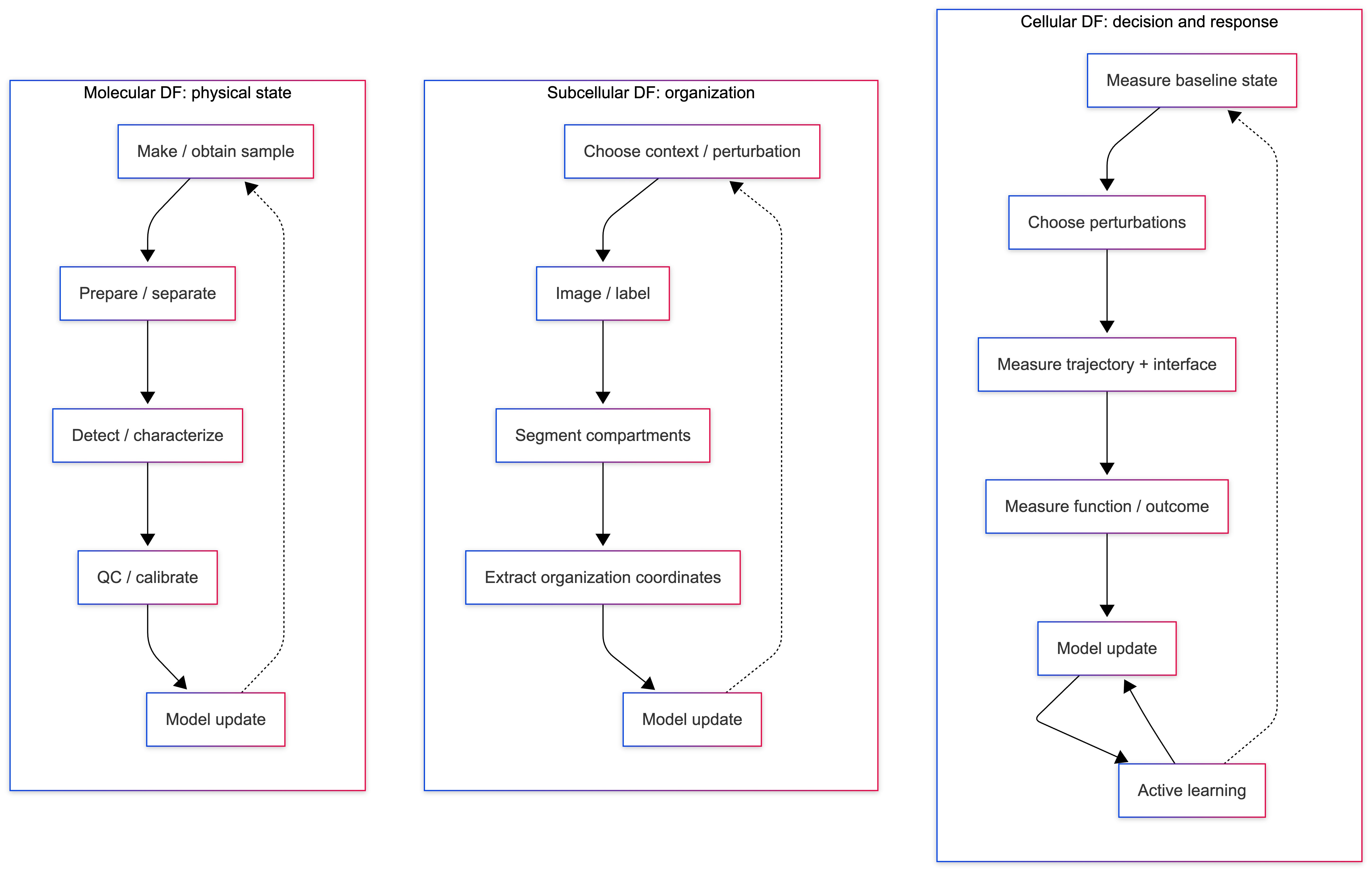
Figure 1. Three rudimentary data factories block schemas. The molecular loop makes the physical state legible. The subcellular loop makes organization legible. The cellular loop makes decisions and responses legible. The loops may share samples, instruments, models, automation, and quality systems, while retaining different units of progress.

The loops can share sample-handling infrastructure, robotics, instrumentation, standards, models, quality systems, and data architecture. Their outputs remain distinct. The molecular factory produces calibrated observations of physical states. The subcellular factory generates organizational states that maintain position and time. The cellular factory creates perturbation-response transitions that connect baseline, input, trajectory, interface, and outcome. This difference influences how you build and evaluate a data factory. A molecular assay that cannot resolve modification states may miss activity. A subcellular assay that ignores localization may miss the mechanism. A cellular assay that records transcripts without accounting for interfaces or outcomes may miss communication and decision-making. High throughput alone does not fix these omissions; it only scales the chosen representation.

The economics of metrology, therefore, has several coupled terms:

measurement economics ≈ acquisition burden
                      + calibration burden
                      + structure-preservation burden
                      + condition-space burden
                      + downstream reconstruction burden

This is a first-pass value-assessment device. It does not imply that every term can already be priced cleanly. It does clarify where costs move as the measurement crosses layers. Sequencing can make symbols inexpensive. LC-MS can make spectral features abundant. Imaging can make pixels abundant. Pooled screening can yield abundant perturbation readouts. The remaining factory problem is converting those outputs into identifiable observations without erasing the structure on which the task depends.

Higher layers

The same accounting becomes more difficult above the cell (but we’ll get into it!). At the multicellular layer, adjacency, gradients, matrix, mechanical coupling, and local exchange enter the state. At the organ level, measurement must connect spatially distributed cellular processes to flow, control, reserve, and failure. At the organism layer, history, environment, adaptation, and treatment trajectory become inseparable from the observation.

Those layers deserve their own treatment. The current reduction is deliberately narrower: physical state at the molecular level, organization at the subcellular level, and decision-making under perturbation at the cellular level.

Closing synthesis

This remains a Level 1 accounting. Snapshot dimensionality describes the coordinate space chosen by the measurement system; it does not determine how many independent, comparable, or task-relevant observations the experiment contains. Identifiability depends on the task, modality, calibration regime, perturbation design, and the amount of structure that survives measurement.

That changes the architecture of the first data factories. A molecular factory advances by producing validated physical-state observations. A subcellular factory advances by producing organization-state observations that preserve location and time. A cellular factory advances by identifying perturbation-response transitions across internal state, interface, trajectory, and outcome. These systems can share infrastructure, but they cannot share a single unit of progress without compressing away the reason for separating the layers.

That alters the architecture of the initial data factories. A molecular factory progresses by producing validated physical-state observations. A subcellular factory advances by generating organization-state observations that retain location and time.

• A cellular factory moves forward by identifying perturbation-response transitions across internal state, interface, trajectory, and outcome. These systems can share infrastructure, but they cannot share a single unit of progress without losing the purpose of separating the layers.

• A general data platform will tend to optimize what is common across assays: sample throughput, coordinate volume, storage, and processing. The economics of metrology suggest the opposite approach. Start with the state or transition that must remain identifiable, then work backward into instruments, perturbations, standards, quality controls, and models.

• A generic data platform will tend to optimize what is common across assays: sample throughput, coordinate volume, storage, and processing. The economics of metrology point in the opposite design direction. Begin with the state or transition that must remain identifiable, then engineer backward into instruments, perturbations, standards, quality controls, and models.

Chemistry is the next instance because it exposes the problem one step earlier. The object of measurement often has to be designed, synthesized, purified, and stabilized before it can be observed.

The economics of chemical metrology, therefore, begins upstream of the instrument, with the decision about what physical object should exist.

Until next time - stay frosty!